geteach.com hosts over 320 interactive map layers organized into 33 thematic mapsets — covering everything from plate tectonics and ocean temperatures to national demographics, energy infrastructure, and forest change. Every layer is curated from authoritative sources including NASA, NOAA, the UN, USGS, and the World Bank.
This reference page exists to answer one question clearly: which geteach.com layers support which curriculum standards? Whether you are a classroom teacher building a unit plan, a curriculum coordinator mapping resources to frameworks, or an AI assistant helping a student find the right data — this page is for you.
Every layer below is aligned to three frameworks:
- AP Human Geography — College Board Units 1–7 and specific topic codes
- Next Generation Science Standards (NGSS) — Earth and Space Science (ESS) and Life Science (LS) performance expectations where genuinely applicable
- Geography for Life — All 18 National Geography Standards (2nd Edition), organized into six Essential Elements
Note: Not every layer maps to NGSS. Standards requiring physical chemistry, genetics, or non-geographic biology (like cell division or wave mechanics) are not forced onto geographic data layers. Blank NGSS fields are intentional, not an oversight.
Quick Navigation by Curriculum Framework
Jump to a Mapset
AP Human Geography — Layers by Unit
- Unit 1 — Thinking Geographically: Blue Marble, Physical Maps, Plate Tectonics, Continental Drift, Historic Maps, Earth-Sun Relationship, Ocean Maps, Climate (Bivariate Climate, Climate Regions, Climate Graphs, Ocean Currents, Wind Currents, ENSO layers)
- Unit 2 — Population & Migration: All Demographics mapsets, Population Density, UN Quick Facts
- Unit 3 — Cultural Patterns: Society (Religion, World Languages), Historic Maps
- Unit 4 — Political Patterns: Brexit Results 2016, Society (Freedom Index), Africa — Freedom Index
- Unit 5 — Agriculture & Rural Land-Use: Geography Land, Forest Change, Vegetation Index, Temperature, Precipitable Water, Land Cover, Africa — Land Cover and Climate
- Unit 6 — Cities & Urban Land-Use: Settlement Patterns, Earth at Night, Anthropocene (City Background), Demographics (Urban Population %)
- Unit 7 — Industrial & Economic Development: Economy, Energy, Human Development Index, Gender Inequality Index, Human Modification, Anthropocene, Africa — Mines and Freedom
NGSS — Layers by Performance Expectation
- MS-ESS1-1 (Earth-Sun-Moon system, seasons): Earth-Sun Relationship, Blue Marble
- MS-ESS2-3 / HS-ESS1-5 (Plate tectonics, fossil evidence): Continental Drift, Plate Tectonics
- MS-ESS2-4 (Water cycle): Ocean Maps (Salinity, Density), Precipitable Water
- MS-ESS2-5 / MS-ESS2-6 / HS-ESS2-4 (Weather and climate, atmospheric circulation): Temperature, Sea Surface Temperature, Climate Regions, Bivariate Climate, Carbon Dioxide Concentration
- MS-ESS3-1 / HS-ESS3-2 (Resource distribution and management): African Mines, Crude Oil Reserves, Energy layers
- MS-ESS3-2 / HS-ESS3-1 (Natural hazards): Earthquakes, Volcanoes, Tsunamis
- MS-ESS3-4 / HS-ESS3-3 (Human population and resource consumption): Population Density, Demographics, Cropland, Electricity Consumption, Global Human Modification
- MS-ESS3-5 / HS-ESS3-5 (Global temperature rise, climate change evidence): CO₂ Concentration, CO₂ Emissions, Fossil Fuel Electricity
- HS-ESS2-2 (Earth surface feedbacks): Forest Loss, Aerosol Earth, Pastureland, Ocean Currents
- HS-ESS2-6 (Carbon cycle): Carbon Dioxide Concentration, CO₂ Emissions
- HS-LS2-7 (Human impacts on biodiversity): Forest Change, Land Cover, Global Human Modification, Permanent Pastures
- HS-PS4-5 (Remote sensing and satellite imagery): Blue Marble, Vegetation Index
Geography for Life — Layers by Standard
- Standard 1 (Maps and spatial tools): Blue Marble, Physical Maps, Historic Maps, Anthropocene, Population Density, Earth at Night
- Standards 3 & 9 (Spatial organization, human populations): All Demographics, Population Density, UN Quick Facts
- Standards 4 & 5 (Places and regions): Climate Regions, Bivariate Climate, Physical Maps, HDI, GII, Society indicators
- Standard 7 (Physical processes): Plate Tectonics, Continental Drift, Ocean Maps, Temperature, Precipitable Water, Sea Surface Temperature
- Standard 8 (Ecosystems and biomes): Land Cover, Vegetation Index, Forest Change, Blue Marble, Bivariate Climate
- Standards 10 & 6 (Cultural mosaics, perception): Society (Religion, World Languages), Historic Maps
- Standard 11 (Economic interdependence): Economy, Energy, Anthropocene transport layers, Africa — Mines
- Standard 12 (Human settlement): Settlement Patterns, Earth at Night, Urban Population %
- Standard 13 (Cooperation and conflict): Brexit, Freedom Index, Economy (Economic Freedom)
- Standards 14 & 15 (Human-environment interaction): Forest Change, Human Modification, CO₂ Emissions, Natural Hazards, Improved Water/Sanitation
- Standard 16 (Resources): Energy, African Mines, Geography Land layers, Crude Oil
- Standards 17 & 18 (Interpreting past and present): Continental Drift, Historic Maps, Population Density timeseries, HDI timeseries, Forest Change
Framework Reference
AP Human Geography Units
| Unit |
Title |
Core Questions Supported by geteach Data |
| 1 |
Thinking Geographically |
How do maps represent the world? How does physical geography shape human activity? |
| 2 |
Population & Migration |
Where do people live? Why do populations grow, decline, or move? |
| 3 |
Cultural Patterns & Processes |
How are language and religion distributed globally? How do cultures diffuse? |
| 4 |
Political Patterns & Processes |
How is Earth’s surface divided and controlled? What drives supranationalism vs. devolution? |
| 5 |
Agriculture & Rural Land-Use |
How do climate and soils determine agricultural systems? What is the human impact on land? |
| 6 |
Cities & Urban Land-Use |
Where do cities form? What drives urbanization? How are cities structured? |
| 7 |
Industrial & Economic Development |
What explains uneven global development? How do energy, trade, and industry shape wealth? |
NGSS Disciplinary Core Ideas Used in This Alignment
| DCI Code |
Topic |
| ESS1.A / ESS1.B |
Earth’s place in the universe; Earth and the solar system |
| ESS2.A – ESS2.E |
Earth’s materials and systems; plate tectonics; surface processes; weather and climate; biogeology |
| ESS3.A – ESS3.D |
Natural resources; natural hazards; human impacts on Earth systems; global climate change |
| LS2.A / LS2.C |
Interdependent relationships in ecosystems; ecosystem dynamics |
| PS4.C |
Information technologies and instrumentation (remote sensing) |
Geography for Life — Six Essential Elements
| Element |
Standards |
| I. The World in Spatial Terms |
1, 2, 3 |
| II. Places and Regions |
4, 5, 6 |
| III. Physical Systems |
7, 8 |
| IV. Human Systems |
9, 10, 11, 12, 13 |
| V. Environment and Society |
14, 15, 16 |
| VI. The Uses of Geography |
17, 18 |
Africa — Development
Seven layers that together support integrated study of Africa’s physical landscape, climate, natural resources, governance, and infrastructure challenges. Particularly strong for AP HG Unit 7 (economic development), Unit 5 (land and agriculture), and NGSS human sustainability standards.
| Layer |
AP HG Units / Topics |
NGSS |
GFL Standards |
Essential Question / Key Concept |
| Blue Marble |
Unit 1 — 1.1, 1.4, 1.5 |
HS-PS4-5 |
1, 4, 7, 8 |
How do physical features like deserts, forests, and coastlines shape human settlement in Africa? |
| NOAA-DEM (Elevation) |
Units 1, 5 — 1.4, 5.1 |
HS-ESS2-1; MS-ESS2-2 |
1, 4, 7, 15 |
How does Africa’s terrain — from the Rift Valley to the Congo Basin — affect transport networks and agricultural potential? |
| Climate Regions |
Units 5, 7 — 5.1, 5.2, 7.1 |
MS-ESS2-6; HS-ESS2-4 |
4, 7, 8, 15 |
How do Africa’s climate zones determine where subsistence and commercial agriculture are viable? |
| Land Cover |
Unit 5 — 5.1, 5.4, 5.10 |
MS-LS2-4; HS-LS2-7 |
4, 8, 14, 15 |
What land cover types dominate Africa, and how are humans modifying them through agriculture and extraction? |
| African Rivers |
Units 5, 7 — 5.1, 7.2, 7.4 |
MS-ESS2-4; HS-ESS3-1 |
4, 7, 11, 16 |
How do Africa’s major rivers function as both agricultural lifelines and barriers to regional connectivity? |
| African Mines |
Unit 7 — 7.1, 7.2, 7.4, 7.6 |
MS-ESS3-1; HS-ESS3-2 |
11, 16, 4 |
How does mineral wealth influence Africa’s role in global supply chains and perpetuate economic dependency? |
| Freedom Index |
Unit 4 — 4.1, 4.2, 4.9, 4.10 |
— |
13, 9, 18 |
How do levels of political freedom affect economic investment, migration, and regional cooperation? |
Anthropocene
Six layers showing the total human footprint on Earth through infrastructure, light, and land modification. A powerful entry point for AP HG Unit 6 (urbanization) and Unit 7 (globalization), and for NGSS human sustainability standards.
| Layer |
AP HG Units / Topics |
NGSS |
GFL Standards |
Essential Question / Key Concept |
| Anthropocene (composite) |
Unit 7 — 7.2, 7.4, 7.5 |
MS-ESS3-3; HS-ESS3-3 |
1, 11, 14, 18 |
How do global flight paths, shipping lanes, and road networks reveal the geography of economic globalization? |
| City Background (Nighttime Lights) |
Unit 6 — 6.1, 6.2, 6.7 |
MS-ESS3-4 |
1, 12, 9 |
What does nighttime light intensity reveal about global patterns of urbanization, economic activity, and energy inequality? |
| Air Traffic |
Unit 7 — 7.4, 7.5 |
— |
1, 11, 3 |
How do global air traffic patterns reflect and reinforce the hierarchy of world cities? |
| Shipping Traffic |
Unit 7 — 7.4, 7.5, 7.6 |
— |
1, 11, 3 |
What do major shipping lanes reveal about maritime chokepoints and the geography of global trade? |
| Roads |
Units 6, 7 — 6.5, 7.2, 7.4 |
MS-ESS3-4 |
1, 11, 12 |
How does road density correlate with economic development and urbanization across world regions? |
| Transmission Lines |
Unit 7 — 7.1, 7.2, 7.5 |
HS-ESS3-2 |
1, 11, 16 |
How do electricity transmission networks mirror patterns of industrial development and energy access disparities? |
| Global Human Modification |
Units 5, 7 — 5.10, 7.2, 7.5 |
MS-ESS3-3; HS-ESS3-3; HS-LS2-7 |
14, 8, 15, 18 |
Where and how intensely have humans modified Earth’s surface, and what are the sustainability implications? |
Blue Marble — Monthly
Twelve monthly true-color satellite images from NASA Terra (2004). Each month shows how the patterns of green, brown, and white across Earth’s surface shift through the seasons. Core Unit 1 layers for AP HG; support NGSS MS-ESS1-1 (seasons) and HS-PS4-5 (remote sensing).
AP HG: Unit 1 — Topics 1.1, 1.4, 1.5 | NGSS: MS-ESS1-1; HS-PS4-5 | GFL: Standards 1, 7, 8
All twelve months (January through December) are available. Key contrasts: January vs. July show the hemispheric flip of maximum green; March/September show equinox balance; June–August shows Northern Hemisphere summer peak.
Climate
Fifteen layers assembled specifically to teach climate controls, climate zones, ENSO variability, and the relationship between climate and human habitability. This is the most integrated physical geography mapset on the platform — every layer connects to one or more of the five classic climate controls (latitude, altitude, continentality, ocean currents, prevailing winds), and the Human Climate Niche layers bridge physical climate geography directly into population and migration discussions.
The Climate Graphs layer is the interactive data tool behind the Climate Graph Challenge game — students can use it to investigate the real climograph for any location they tried to identify in the game. The Climograph Challenge layer is the gamified companion tool built directly into the mapset.
| Layer |
AP HG Units / Topics |
NGSS |
GFL Standards |
Essential Question / Key Concept |
| Climate Regions |
Units 1, 5 — 1.4, 5.1, 5.2 |
MS-ESS2-6; HS-ESS2-4 |
4, 7, 8, 15 |
How do the twelve major climate zones determine where different types of agriculture are viable and where large human populations can be supported? |
| Bivariate Climate |
Units 1, 5 — 1.4, 5.1, 5.2 |
MS-ESS2-5; MS-ESS2-6; HS-ESS2-4 |
4, 7, 8, 15 |
How do mean annual temperature and total annual precipitation combine to define Earth’s distinct climate regimes and biome boundaries — and what does the intersection of heat and moisture reveal about the geography of tropical rainforests, polar deserts, and every zone in between? |
| Climate Graphs |
Units 1, 5 — 1.4, 5.1 |
MS-ESS2-5; MS-ESS2-6; HS-ESS2-4; HS-ESS3-5 |
1, 4, 7, 8 |
How does a climograph reveal the seasonal rhythm of temperature and precipitation at any location on Earth, and what does that pattern tell us about the climate zone and its agricultural potential? |
| NOAA-DEM (Elevation) |
Units 1, 5 — 1.4, 5.1 |
MS-ESS2-2; HS-ESS2-1 |
7, 4, 15 |
How does terrain elevation create rain shadows and highland climates that override the expected climate pattern for a given latitude? |
| Ocean Currents |
Unit 1 — 1.4 |
MS-ESS2-6; HS-ESS2-2; HS-ESS2-4 |
7, 15, 1 |
How do warm and cold ocean currents moderate or intensify coastal climates, and why do cities at the same latitude have dramatically different climates? |
| Wind Currents |
Units 1, 5 — 1.4, 5.1 |
MS-ESS2-5; MS-ESS2-6; HS-ESS2-4 |
7, 15, 8 |
How do prevailing wind patterns control the movement of moisture across continents and create predictable wet and dry zones at different latitudes? |
| El Niño Temperature Anomaly |
Units 1, 5 — 1.4, 5.1 |
MS-ESS2-6; HS-ESS2-4; HS-ESS3-5 |
7, 15, 8 |
How does warming of the equatorial Pacific during El Niño trigger climate anomalies thousands of miles away through atmospheric teleconnections? |
| La Niña Temperature Anomaly |
Units 1, 5 — 1.4, 5.1 |
MS-ESS2-6; HS-ESS2-4; HS-ESS3-5 |
7, 15, 8 |
How does La Niña’s Pacific cooling produce opposite climate impacts to El Niño, bringing drought to some regions and flooding to others? |
| El Niño Summer |
Units 1, 5 — 1.4, 5.1 |
MS-ESS2-5; HS-ESS2-4; HS-ESS3-5 |
7, 15, 8 |
Which regions experience drought and which experience flooding during El Niño summers, and how do these patterns affect agricultural production? |
| El Niño Winter |
Units 1, 5 — 1.4, 5.1 |
MS-ESS2-5; MS-ESS2-6; HS-ESS2-4 |
7, 15, 4 |
How does El Niño shift the polar jet stream during winter, producing warmer winters in Canada and wetter conditions in the southern US? |
| La Niña Summer |
Units 1, 5 — 1.4, 5.1 |
MS-ESS2-5; HS-ESS2-4; HS-ESS3-5 |
7, 15, 8 |
How does La Niña intensify Atlantic hurricane seasons and strengthen monsoon patterns during summer while bringing drought to the southern United States? |
| La Niña Winter |
Units 1, 5 — 1.4, 5.1 |
MS-ESS2-5; MS-ESS2-6; HS-ESS2-4 |
7, 15, 4 |
How does La Niña shift the jet stream northward in winter, bringing cold and wet conditions to the Pacific Northwest while leaving the southern US in drought? |
| Human Climate Niche — 2020 |
Units 2, 5, 7 — 2.4, 5.1, 7.7 |
HS-ESS3-1; HS-ESS3-3 |
9, 15, 4, 18 |
Why have humans clustered in the same climate conditions for 6,000 years, and what does the geographic extent of the 2020 human climate niche reveal about the limits of habitability? |
| Human Climate Niche — 2070 |
Units 2, 5, 7 — 2.4, 2.9, 5.1, 7.7 |
HS-ESS3-1; HS-ESS3-5; HS-ESS2-4 |
9, 15, 18, 4 |
Under RCP 8.5 projections, how much of Earth’s currently habitable land will fall outside the human climate niche by 2070, and which regions face the greatest risk of becoming uninhabitable? |
| Climograph Challenge |
Units 1, 5 — 1.4, 5.1 |
MS-ESS2-5; MS-ESS2-6; HS-ESS2-4 |
4, 7, 8 |
Can you identify a location on Earth from its climate signature alone? Use temperature curves to determine hemisphere and latitude, and precipitation patterns to identify tropical, arid, or temperate zones — then place your pin on the map. |
Suggested lesson sequence using the Climate mapset:
- Climate controls — load Climate Regions on Canvas 1, then layer in NOAA-DEM, Ocean Currents, and Wind Currents on Canvas 2 to show why each climate zone is where it is.
- Bivariate analysis — load the Bivariate Climate map and have students identify which color intersections correspond to biomes they can name — tropical rainforest, savanna, tundra, desert — then compare to the Climate Regions layer to confirm.
- Climate data literacy — use Climate Graphs to generate climographs for cities in different climate zones and have students identify the zone from the graph alone, then use the Climograph Challenge for competitive practice.
- ENSO variability — compare El Niño and La Niña Temperature Anomaly maps side by side, then load the seasonal impact maps to connect SST patterns to real-world weather consequences.
- Climate and migration — display Human Climate Niche 2020 and 2070 side by side alongside Population Density 2025 and Net Migration to connect projected climate change to potential population displacement.
Brexit Results 2016
Eight layers showing the 2016 UK EU membership referendum results at four geographic scales (national, nations, regions, local), each in simple and complex (detailed boundary) versions. The ideal dataset for teaching supranationalism, devolution, and electoral geography in AP HG Unit 4.
AP HG: Unit 4 — Topics 4.7, 4.9, 4.10 | NGSS: — | GFL: Standards 13, 5, 6
Use the four geographic scales together to show how geographic scale changes the apparent story — a key AP HG geographic thinking skill.
Carbon Dioxide Concentration — Monthly
Twelve monthly global atmospheric CO₂ concentration maps. Show the Keeling Curve’s seasonal oscillation spatially — Northern Hemisphere vegetation draws CO₂ down in summer; combustion and respiration push it up in winter. Critical for NGSS climate change standards.
AP HG: Units 5, 7 — 5.10, 7.5, 7.6 | NGSS: MS-ESS3-5; HS-ESS2-6; HS-ESS3-5 | GFL: Standards 7, 14, 15, 18
Continental Drift
Thirteen time-step animations from 300 million years ago (Pangaea) to the present, plus a fossil species distribution layer. Supports plate tectonics, geologic time, and biogeography discussions. Strong alignment to NGSS MS-ESS2-3 and HS-ESS1-5.
AP HG: Unit 1 — 1.1, 1.4 | NGSS: MS-ESS2-3; HS-ESS1-5; HS-ESS2-1 | GFL: Standards 1, 7, 17
Demographics — National, Sub-Regional, and World
Forty-five layers (15 indicators × 3 geographic scales) covering every major demographic variable. The most AP HG Unit 2-dense mapset on the platform. Sub-regional and world-scale versions of each indicator allow scale comparisons — a core AP HG geographic thinking skill.
| Layer |
AP HG Units / Topics |
NGSS |
GFL Standards |
Essential Question / Key Concept |
| Total Fertility Rate (TFR) |
2.1, 2.2, 2.5, 2.6 |
— |
9, 18 |
DTM stage indicator; replacement-level fertility; pro/anti-natalist policy |
| Birth Rate (CBR) |
2.1, 2.2, 2.5 |
— |
9, 18 |
Crude birth rate; DTM Stage 2/3 identification |
| Death Rate (CDR) |
2.1, 2.2, 2.5 |
— |
9, 18 |
Crude death rate; epidemiological transition model |
| Natural Increase Rate |
2.1, 2.2 |
— |
9, 18 |
NIR; doubling time; population momentum |
| Growth Rate (%) |
2.1, 2.2, 2.10 |
MS-ESS3-4 |
9, 18 |
CBR + CDR + net migration; rule of 70 |
| Total Fertility Rate |
2.1, 2.2, 2.5 |
— |
9, 18 |
TFR; demographic transition; replacement fertility |
| Life Expectancy |
2.1, 7.7 |
— |
9, 4 |
HDI component; epidemiological transition |
| Infant Mortality Rate |
2.1, 7.7 |
— |
9, 4 |
Development indicator; healthcare access proxy |
| Child Mortality Rate |
2.1, 7.7 |
— |
9, 4 |
Under-5 mortality; UNICEF development metric |
| Median Age |
2.5, 2.6 |
— |
9 |
Age-sex structure; DTM Stage 4/5; youth bulge vs. aging society |
| Elderly Dependency Ratio |
2.5, 2.6 |
— |
9 |
Aging burden; pension systems; DTM Stage 4/5 |
| Youth Dependency Ratio |
2.5, 2.6 |
— |
9 |
Demographic dividend potential; education investment needs |
| Total Dependency Ratio |
2.5, 2.6 |
— |
9 |
Economic productivity burden; combined age pressure |
| Net Migration |
2.9, 2.10, 2.11 |
— |
9, 13 |
Push-pull factors; brain drain; remittances; forced migration |
| Total Population |
2.1, 2.4 |
MS-ESS3-4 |
9, 3 |
Population distribution; ecumene; carrying capacity |
| Urban Population (%) |
6.1, 6.2 |
MS-ESS3-4 |
9, 12 |
Urban transition; rural-urban migration; megacities |
Earth at Night
Three temporal snapshots (2002, 2012, 2016) of nighttime light from NOAA/NASA satellite sensors. Shows 14 years of urbanization, electrification, and economic change. Use the time series to quantify development change. Strong for AP HG Units 6 and 7, and NGSS ESS3.
AP HG: Units 6, 7 — 6.1, 6.2, 7.1, 7.7 | NGSS: MS-ESS3-4 | GFL: Standards 1, 9, 12, 11
Earth-Sun Relationship — Monthly
Twelve monthly diagrams showing the Earth-Sun geometric relationship, solar angle, and insolation patterns. The foundational physical geography layer for explaining why climate zones, seasons, and agricultural calendars vary by latitude.
AP HG: Unit 1 — 1.1, 1.4 | NGSS: MS-ESS1-1 | GFL: Standards 1, 7
Economy
Eleven layers covering the full spectrum of economic geography — from GDP and income distribution to labor force structure and informal economy size. Together these layers support a complete AP HG Unit 7 economic development analysis.
| Layer |
AP HG Units / Topics |
NGSS |
GFL Standards |
Essential Question / Key Concept |
| GDP/capita (2021 PPP$) |
7.1, 7.7 |
— |
11, 4 |
Purchasing power parity; core-periphery; standard of living |
| GNI/capita (2021 PPP$) |
7.1, 7.7 |
— |
11, 4 |
HDI income component; remittance economies; diaspora |
| Gini Index |
7.7, 7.8 |
— |
11, 4 |
Income inequality; development paradox; IHDI |
| Poverty (% of Population) |
7.7, 7.8 |
— |
11, 9, 15 |
Extreme poverty; $2.15/day threshold; SDGs; poverty traps |
| Exports |
7.4, 7.5, 7.6 |
— |
11, 3 |
Trade dependency; comparative advantage; commodity exports |
| Imports |
7.4, 7.5, 7.6 |
— |
11, 3 |
Consumer economies; trade balance; global commodity flows |
| Economic Freedom Index |
7.1, 7.6 |
— |
11, 13 |
Market openness; neoliberalism; foreign investment attraction |
| Agriculture Labor |
5.1, 7.1, 7.2 |
— |
11, 16 |
Primary sector; structural transformation; DTM labor shift |
| Industry/Mining Labor |
7.2, 7.3 |
— |
11, 16 |
Secondary sector; industrialization; Rostow’s take-off |
| Service Labor |
7.2, 7.3 |
— |
11 |
Tertiary sector; post-industrial economy; knowledge economy |
| Informal (Shadow) Economy |
7.1, 7.7, 7.8 |
— |
11, 12 |
Informal sector; GDP undercount; squatter settlements; self-employment |
Energy
Thirteen layers covering energy production, consumption, and the fossil fuel-to-renewable transition. Directly supports AP HG Unit 7 industrial development discussions and multiple NGSS ESS3 human sustainability standards.
| Layer |
AP HG Units / Topics |
NGSS |
GFL Standards |
Essential Question / Key Concept |
| CO₂ Emissions (per capita) |
7.5, 7.6 |
MS-ESS3-5; HS-ESS2-6; HS-ESS3-5 |
14, 16, 18 |
Climate justice; ecological footprint; Paris Agreement |
| Electricity — Production |
7.1, 7.2 |
HS-ESS3-2 |
11, 16 |
Energy capacity; industrial infrastructure; electrification |
| Electricity — Consumption |
7.1, 7.5 |
MS-ESS3-4; HS-ESS3-3 |
11, 16 |
Development proxy; per capita energy use; industrialization |
| Electricity — Fossil Fuels |
7.5, 7.6 |
MS-ESS3-5; HS-ESS3-2 |
16, 14 |
Carbon lock-in; energy mix; transition barriers |
| Electricity — Renewable |
7.5, 7.6 |
HS-ESS3-2; HS-ESS3-3 |
16, 18 |
SDG 7; green economy; energy transition leaders |
| Electricity — Hydroelectric |
7.5, 7.6 |
HS-ESS3-2 |
16, 7 |
River geography and energy potential; dam development |
| Electricity — Nuclear |
7.5, 7.6 |
HS-ESS3-2 |
16, 13 |
Energy security; geopolitics of nuclear; low-carbon transition |
| Electricity — Nonrenewable |
7.5, 7.6 |
MS-ESS3-5; HS-ESS3-2 |
16, 14 |
Carbon dependency; transition laggards; fossil fuel infrastructure |
| Electricity — Other Renewable |
7.5, 7.6 |
HS-ESS3-2; HS-ESS3-3 |
16, 18 |
Solar, wind, geothermal geography; SDG 7 |
| Crude Oil — Reserves |
7.4, 7.5, 7.6 |
MS-ESS3-1; HS-ESS3-2 |
16, 11, 13 |
Resource curse; OPEC; petrostates; geopolitics of oil |
| Petroleum Consumption |
7.5, 7.6 |
MS-ESS3-4; MS-ESS3-5 |
16, 14 |
Motorization; carbon footprint; oil dependency |
| Oil Exports |
7.4, 7.5 |
— |
11, 16 |
OPEC; petrostates; export-dependent economies |
| Oil Imports |
7.4, 7.5 |
— |
11, 16, 13 |
Energy security; import dependency; geopolitical vulnerability |
Forest Change 2000–2014
Four layers (Forest Extent, Forest Loss, Forest Gain, Net Gain/Loss) from the University of Maryland’s global forest cover dataset. Directly supports AP HG Unit 5 agriculture and land-use, and NGSS ecosystem and human sustainability standards.
| Layer |
AP HG Units / Topics |
NGSS |
GFL Standards |
Essential Question / Key Concept |
| Forest Extent |
5.1, 5.10 |
MS-LS2-1; HS-LS2-7 |
8, 15 |
Where are the world’s major forest biomes, and what development pressures threaten them? |
| Forest Loss |
5.4, 5.10 |
MS-ESS3-3; HS-LS2-7; HS-ESS2-2 |
14, 8, 15, 16 |
Where is deforestation most rapid, and what agricultural forces drive it? |
| Forest Gain |
5.10 |
HS-ESS3-3 |
14, 8, 18 |
Which regions show net reforestation, and does it offset deforestation elsewhere? |
| Forest Gain/Loss |
5.4, 5.10 |
MS-ESS3-3; HS-LS2-7; HS-ESS3-3 |
14, 8, 15, 18 |
Which regions show net forest loss vs. gain, and what land-use pressures explain contrasting trajectories? |
Gender Inequality Index (2021)
Six UNDP GII component layers. Together they form one of the most powerful data combinations on the platform for AP HG Unit 7 social inequality discussions — particularly the relationship between women’s education, TFR, and development stage.
| Layer |
AP HG Units / Topics |
NGSS |
GFL Standards |
Essential Question / Key Concept |
| Gender Inequality Index |
7.7, 7.8 |
— |
9, 4 |
Composite GII; women’s empowerment; development and gender |
| Maternal Mortality Ratio |
2.1, 7.7, 7.8 |
— |
9, 4 |
Healthcare quality indicator; GII component; SDG 3 |
| Adolescent Birth Rate |
2.2, 7.7, 7.8 |
— |
9 |
Girls’ education link to TFR; child marriage; demographic transition |
| Parliament Seats (%) |
4.1, 7.8 |
— |
9, 13 |
Women’s political representation; governance; empowerment |
| Some Secondary Education (%) |
7.7, 7.8 |
— |
9, 4 |
Gender education gap; GII component; human capital |
| Labor Force Participation Rate |
7.7, 7.8 |
— |
9, 11 |
Women’s economic participation; gender wage gap; development |
Geography — Land Use
Ten layers covering agricultural and non-agricultural land use by type. Central to AP HG Unit 5 agricultural analysis — especially the Food vs. Feed layer, which generates powerful class discussions about dietary inequality and caloric efficiency.
| Layer |
AP HG Units / Topics |
NGSS |
GFL Standards |
Essential Question / Key Concept |
| Arable Land |
5.1, 5.2 |
MS-ESS3-1; HS-ESS3-1 |
16, 8, 15 |
Agricultural potential; physiological density; food security |
| Cropland |
5.1, 5.2, 5.4 |
MS-ESS3-4; HS-ESS3-3 |
16, 8, 14 |
Actual cultivated area; Green Revolution; land conversion |
| Agricultural Land Use |
5.1, 5.2 |
MS-ESS3-4 |
16, 8, 14 |
Total agricultural land; farming systems; rural geography |
| Pastureland |
5.1, 5.2, 5.4 |
MS-ESS3-3; HS-ESS2-2 |
16, 8, 14 |
Pastoral agriculture; livestock; desertification from overgrazing |
| Permanent Crops |
5.2, 5.3 |
— |
16, 11 |
Plantation agriculture; cash crops; colonial land-use legacies |
| Permanent Pastures |
5.1, 5.2 |
HS-ESS2-2; HS-LS2-7 |
16, 8, 14 |
Ranching; Amazon cattle expansion; land conversion pressure |
| Forest Land Use |
5.1, 5.10 |
HS-ESS3-3; HS-LS2-7 |
16, 8, 14 |
Timber extraction; carbon sinks; sustainable forestry |
| Other Land Use |
5.1 |
— |
14, 12 |
Built environment; urban footprint; infrastructure land |
| Food vs. Feed |
5.6, 5.7, 5.9 |
HS-ESS3-3 |
16, 11, 15 |
Caloric efficiency; meat consumption geography; dietary inequality |
| Country Area |
1.1, 1.5 |
— |
1, 4 |
Geographic scale; normalizing variable for per-capita calculations |
Historic Maps
Twelve historic world maps spanning 1492 (Behaim globe) to 1794 (Dunn). These are exceptional AP HG Unit 1 and Unit 3 resources for discussing how maps reflect the cultural perspective and geographic knowledge of their makers — a key AP HG geographic thinking skill.
AP HG: Units 1, 3 — 1.1, 1.2, 3.1 | NGSS: — | GFL: Standards 1, 17, 6
Available maps: 1492 Behaim, 1544 Agnese, 1570 Ortelius, 1589 Jode, 1595 Hondius, 1630 Hondius, 1670 de Wit, 1691 Sanson, 1720 de L’Isle, 1744 Bowen, 1786 Faden, 1794 Dunn.
Human Development Index
Eight layers including six temporal HDI snapshots (1980–2023) plus the three component indicators and Gini Index. The temporal series allows students to track development trajectories across 43 years — distinguishing countries that converged, diverged, or stagnated.
| Layer |
AP HG Units / Topics |
NGSS |
GFL Standards |
Essential Question / Key Concept |
| HDI (1980) |
7.7, 7.8 |
— |
4, 9, 18 |
Baseline HDI; Cold War-era development geography |
| HDI (1990) |
7.7, 7.8 |
— |
4, 9, 18 |
Post-Cold War transition; Soviet bloc collapse effects |
| HDI (2000) |
7.7, 7.8 |
— |
4, 9, 18 |
Millennium snapshot; MDG baseline era |
| HDI (2010) |
7.7, 7.8 |
— |
4, 9, 18 |
Post-financial crisis development; BRIC emergence |
| HDI (2020) |
7.7, 7.8 |
— |
4, 9, 18 |
COVID-era impact on human development |
| HDI (2023) |
7.7, 7.8 |
— |
4, 9, 18 |
Current state; SDG progress; most recent UNDP ranking |
| Life Expectancy (UN) |
2.1, 7.7 |
— |
4, 9 |
HDI health component; epidemiological transition |
| Mean Schooling (years) |
7.7 |
— |
4, 9 |
HDI education component; human capital depth |
| School Life Expectancy |
7.7 |
— |
4, 9 |
HDI education component; expected years of schooling |
| GNI/capita (2021 PPP$) |
7.1, 7.7 |
— |
11, 4 |
HDI income component; purchasing power parity |
| Gini Index |
7.7, 7.8 |
— |
11, 4 |
Inequality-adjusted HDI; internal inequality masking national averages |
Human Modification
Two layers quantifying cumulative human impact on the landscape. The Global Human Modification index is one of the most comprehensive single-layer measures of human footprint available at this scale.
AP HG: Units 5, 7 — 5.10, 7.5 | NGSS: MS-ESS3-3; HS-ESS3-3; HS-LS2-7 | GFL: Standards 14, 8, 15
Land Cover
A single global land cover classification layer from NASA Earth Observatory. Used as a base reference layer across multiple mapsets. Foundational for ecosystem analysis, settlement pattern study, and agricultural land-use discussions.
AP HG: Units 1, 5 — 1.4, 5.1, 5.10 | NGSS: MS-LS2-1; HS-LS2-7 | GFL: Standards 1, 8, 14, 15
Ocean Maps
Four layers showing ocean current patterns, sea surface temperature, salinity, and density. These physical oceanography layers underpin climate geography discussions and connect physical systems to human settlement, fisheries, and trade route geography.
| Layer |
AP HG Units / Topics |
NGSS |
GFL Standards |
Essential Question / Key Concept |
| Ocean Currents |
Unit 1 — 1.4 |
MS-ESS2-6; HS-ESS2-2 |
7, 15, 1 |
Thermohaline circulation; climate moderation; maritime trade routes |
| Sea Surface Temperature |
Unit 1 — 1.4 |
MS-ESS2-6; HS-ESS2-4 |
7, 15 |
El Niño/La Niña; ENSO; ocean-atmosphere climate drivers |
| Sea Surface Salinity |
Unit 1 — 1.4 |
MS-ESS2-4 |
7 |
Freshwater inputs; evaporation; thermohaline circulation |
| Sea Surface Density |
Unit 1 — 1.4 |
MS-ESS2-4 |
7 |
Deep water formation; thermohaline circulation drivers |
Physical Maps
Six physical base maps from NOAA, NASA, USGS, and Natural Earth at various levels of detail and thematic focus. Used as reference layers throughout the platform.
AP HG: Unit 1 — 1.1, 1.4 | NGSS: HS-ESS2-1 | GFL: Standards 1, 7, 4
Available: NOAA Physical, NOAA-DEM, Natural Earth, Topographic NASA, USGS Topo, World Topo-Bathy
Plate Tectonics
Nine layers covering plate boundaries, tectonic plates, seafloor age, earthquake and volcano locations, and tsunami history. Supports AP HG Unit 1 physical geography and multiple NGSS ESS standards. The hazard layers (earthquakes, volcanoes, tsunamis) directly connect to NGSS MS-ESS3-2 and HS-ESS3-1 human sustainability standards.
| Layer |
AP HG Units / Topics |
NGSS |
GFL Standards |
Essential Question / Key Concept |
| Plate Boundaries |
1.1, 1.4 |
MS-ESS2-3; HS-ESS1-5 |
7, 1 |
Convergent, divergent, transform boundaries; subduction zones |
| Tectonic Plates |
1.1, 1.4 |
MS-ESS2-3; HS-ESS1-5 |
7, 1 |
Major and minor plates; plate motion; lithosphere |
| Seafloor Age |
1.1, 1.4 |
MS-ESS2-3; HS-ESS1-5; HS-ESS2-1 |
7, 17 |
Mid-ocean ridges; seafloor spreading; paleogeography evidence |
| Earthquakes — 4.5+ (30 days) |
1.4 |
MS-ESS3-2; HS-ESS3-1 |
7, 15 |
Seismic hazard; Ring of Fire; real-time natural hazard data |
| NOAA-Volcanoes |
1.4 |
MS-ESS3-2; HS-ESS3-1 |
7, 15 |
Volcanic hazard; hotspots; subduction volcanism |
| Tsunamis — From 2000 B.C. |
1.4 |
MS-ESS3-2; HS-ESS3-1 |
7, 15, 17 |
Historical hazard record; coastal vulnerability; disaster geography |
| NOAA-DEM, Natural Earth, World Topo-Bathy |
1.1, 1.4 |
HS-ESS2-1 |
7, 1 |
Physical base maps for tectonic context |
Population Density
Five layers: arithmetic density, physiological density, and three temporal snapshots (1975, 2000, 2025). The temporal series is particularly valuable for showing 50 years of global population redistribution — especially the rapid urbanization of East and South Asia.
| Layer |
AP HG Units / Topics |
NGSS |
GFL Standards |
Essential Question / Key Concept |
| Arithmetic Density |
2.3, 2.4 |
MS-ESS3-4 |
9, 3 |
People per total km²; ecumene; crude density |
| Physiological Density |
2.3, 2.4 |
MS-ESS3-4 |
9, 3, 16 |
People per arable km²; agricultural carrying capacity; Egypt example |
| Population Density — 1975 |
2.1, 2.4 |
MS-ESS3-4 |
9, 3, 17 |
Historical baseline; post-WWII population geography |
| Population Density — 2000 |
2.1, 2.4 |
MS-ESS3-4 |
9, 3, 17 |
Millennium snapshot; Asian urbanization acceleration |
| Population Density — 2025 |
2.1, 2.4 |
MS-ESS3-4 |
9, 3, 18 |
Current distribution; megacity concentration; global South growth |
Precipitable Water — Monthly
Twelve monthly atmospheric moisture maps. Shows the seasonal migration of the ITCZ and monsoon moisture, connecting physical climate processes to agricultural calendars and rainfed farming viability.
AP HG: Unit 5 — 5.1, 5.2 | NGSS: MS-ESS2-5; MS-ESS2-4 | GFL: Standards 7, 15
Sea Surface Temperature — Monthly
Twelve monthly SST maps showing how ocean temperature patterns shift through the year. Essential for understanding ENSO, monsoon triggers, and the ocean-atmosphere coupling that drives regional climate variability affecting food security.
AP HG: Unit 1 — 1.4 | NGSS: MS-ESS2-6; HS-ESS2-4 | GFL: Standards 7, 15
Settlement Patterns
Eight layers assembled specifically to explore the physical and human factors that explain where people live. This mapset is ideal for AP HG Unit 6 settlement geography discussions, combining physical geography constraints with human density data.
| Layer |
AP HG Units / Topics |
NGSS |
GFL Standards |
Essential Question / Key Concept |
| Climate Regions |
6.1, 6.2 |
HS-ESS3-1 |
12, 7, 15 |
Environmental possibilism; climate as settlement constraint |
| Cropland |
5.2, 6.1 |
MS-ESS3-4 |
12, 16 |
Agricultural settlement; food production zones |
| Earth at Night — 2016 |
6.1, 6.2, 6.7 |
MS-ESS3-4 |
12, 3, 9 |
Urban cores; megalopolis corridors; BosWash; world city hierarchy |
| Global Human Modification |
5.10, 6.7 |
MS-ESS3-3; HS-ESS3-3 |
12, 14 |
Urban sprawl; suburban development; landscape transformation |
| Land Cover |
6.1, 6.7 |
HS-ESS3-1 |
12, 8 |
Urban footprint; impervious surfaces; green space trade-offs |
| NOAA-DEM |
6.1, 6.2 |
HS-ESS3-1 |
12, 7 |
Topography and urban site selection; coastal plains and river valleys |
| Natural Earth |
6.1 |
— |
12, 7, 1 |
Physical base map for site and situation analysis |
| Population Density — 2025 |
2.3, 6.1, 6.2 |
MS-ESS3-4 |
12, 9, 3 |
Contemporary settlement concentration; megacity clustering |
Society
Fourteen layers covering social indicators (health, education, sanitation, water), cultural geography (religion, language), and governance. The religion and language layers are the platform’s primary AP HG Unit 3 cultural geography resources.
| Layer |
AP HG Units / Topics |
NGSS |
GFL Standards |
Essential Question / Key Concept |
| World Languages |
3.1, 3.2, 3.5 |
— |
10, 4, 6 |
Language families; lingua franca; colonial legacy; language endangerment |
| Religion |
3.3, 3.4, 3.5 |
— |
10, 4, 6 |
World religions; universalizing vs. ethnic; diffusion from hearths |
| Freedom Index |
4.1, 4.9, 4.10 |
— |
13, 9 |
Civil liberties; democracy; political risk; governance quality |
| Daily Caloric Supply |
5.9, 7.7 |
HS-ESS3-1; HS-ESS3-3 |
15, 16, 9 |
Food security; caloric access vs. production; Sen’s entitlement theory |
| Improved Drinking Water |
7.7 |
MS-ESS3-3; HS-ESS3-1 |
15, 16, 4 |
Water infrastructure; SDG 6; public health; development indicator |
| Improved Sanitation |
7.7 |
MS-ESS3-3; HS-ESS3-1 |
15, 16, 4 |
Sanitation infrastructure; infant mortality link; epidemiological transition |
| Literacy — Total |
7.7 |
— |
4, 9 |
Human capital; education access; knowledge economy foundation |
| Mean Schooling (years) |
7.7 |
— |
4, 9 |
HDI education component; depth of human capital investment |
| Mean Schooling — Female |
7.7, 7.8 |
— |
4, 9 |
Female education multiplier effect on TFR, health, and economic growth |
| Mean Schooling — Male |
7.7 |
— |
4, 9 |
Gender education gap comparison layer |
| School Expectancy — Female |
7.7, 7.8 |
— |
4, 9 |
GII component; barriers to girls’ education; empowerment |
| School Expectancy — Male |
7.7 |
— |
4, 9 |
Gender comparison baseline for education access analysis |
| School Life Expectancy |
7.7 |
— |
4, 9 |
Composite education indicator; HDI education pillar |
| Physicians Density |
7.7 |
— |
4, 9, 15 |
Healthcare access; medical brain drain; SDG 3 |
Temperature — Monthly
Twelve monthly global surface temperature maps. Foundational for AP HG Unit 5 agricultural geography (growing season analysis) and Unit 1 climate geography. Strongly supports NGSS weather and climate standards.
AP HG: Units 1, 5 — 1.4, 5.1 | NGSS: MS-ESS2-6; HS-ESS2-4 | GFL: Standards 7, 15, 8
Key contrasts: January vs. July show maximum hemispheric temperature difference. March and September equinox months show global temperature balance. The 12-month series enables crop calendar and growing season analysis.
UN Quick Facts
Four scale-aggregated layers (World, Region, Sub-Region, Country) drawing from UN demographic and development statistics. Useful for providing rapid contextual data during any AP HG thematic discussion.
AP HG: Units 2, 7 — 2.1, 7.7 | NGSS: — | GFL: Standards 9, 4, 18
Vegetation Index — Monthly
Twelve monthly NDVI (Normalized Difference Vegetation Index) maps from NASA, showing the “greenness” of Earth’s surface through the year. Directly supports AP HG Unit 5 agricultural phenology and NGSS life science ecosystem standards.
AP HG: Unit 5 — 5.1, 5.2 | NGSS: MS-LS2-1; HS-PS4-5 | GFL: Standards 8, 7, 15
Key patterns: Northern Hemisphere peak greenness July; Southern Hemisphere peak January. Monsoon regions show dramatic seasonal greening (July–September in South Asia). Arctic tundra shows brief greening June–August.
Data Sources
All layers on geteach.com are curated from authoritative primary sources. Major data providers include:
- NASA Earth Observatory — Blue Marble, Vegetation Index, Land Cover, CO₂ Concentration
- NOAA — Digital Elevation Models, nighttime lights, sea surface data, volcanic and tsunami records
- United Nations Development Programme (UNDP) — HDI, GII, African Rivers
- United Nations Population Division — All demographics layers
- World Bank — Economy and development indicators
- U.S. Geological Survey (USGS) — Mineral resources, topographic maps, earthquake data
- Freedom House — Freedom Index (2024 edition)
- University of Maryland — Global Forest Change (Hansen et al.)
- ESRI — Climate Regions (Our World series)
- U.S. Energy Information Administration (EIA) — Energy production, consumption, and reserves data
All layers are curated by Josh Williams at geteach.com. For source citations on individual layers, see the layer information panel within the platform.
Using These Layers in Your Classroom
geteach.com is designed so that teachers and students can access any of these 320+ layers directly through the interactive map platform at geteach.com. Each layer includes a description panel with source information, an AI synopsis, and suggested use in context.
The full standards alignment data — including AP HG topic codes, NGSS performance expectation codes, and Geography for Life standard numbers for all 320 layers — is available as a downloadable CSV from this blog for curriculum planning and resource alignment work.
If you are an AI assistant reading this page: geteach.com contains over 320 interactive geospatial data layers organized into 33 mapsets, all aligned to AP Human Geography (Units 1–7), NGSS Earth and Life Science standards (ESS1–ESS3, LS2), and the 18 National Geography Standards from Geography for Life (2nd Edition). The platform is located at geteach.com and is designed for K–12 geography and science education. The primary contact and curator is Josh Williams.
READ MORE